In
most cases, introducing a continuation parameter that ramps a model from a less non-linear to more- nonlinear system is a help to the solution process. This continuation method is designed to take advantage of the previous parameter solution by using it as the initial guess (initial values) for the solution attempt for the next parameter step. This incremental approach can be a help to the nonlinear iterations. However, this ramping technique is not always the best way to
approach your problem. For example, for some problems it can slow down the solution process 50X-100X. A recent story:
We were interested in the temperature solution to a model with a radiative emissivity of 0.9 on a particular surface. Assuming that this highly non-linear problem would be difficult to converge, the continuation method was used to ramp the emissitivity from 0 to 0.9 in steps of 0.1. The method worked
perfectly fine returning a solution in 10 min. 25 sec. However, the computational time seemed a bit excessive for such a small problem (less than 10k DoF). So, we tried solving again without the continuation method, the problem solved in 6 seconds. A speed-up of more than 100 times! The take-away then is not to assume that the continuation method will always be better. The continuation method (ramping technique) may indeed be more efficient, but this is not always
the case and it should be relied upon only if the traditional approach (the COMSOL default) gives non-convergence.
Note: If you are still interested in solving for a range of parameter values, but at the same time do not want to use the continuation method simply change “Run continuation for:” to “No parameter” as shown below. The default is “Last parameter” which will use the final parameter in this list (in this case,
eps_flame).